This chapter is intended to give a basic introduction to the classical theory of volume diffusion.

Bibliography to this section and further details and aspects can be found in [ErdelyiPhD].

2.1 Fick’s equations

Diffusion of atoms in solids can be described by the Fick’s equations. The first equation relates the flux ($$\vec{j}$$: number of atoms crossing a unit area per unit time) to the gradient of the concentration ($$\rho$$: number of atoms per unit volume) via the diffusion coefficient tensor $$\hat{D}$$:

\begin{equation}
\vec{j}=-\hat{D}\mathrm{grad}\rho. \label{eq:vector_Fick_I}
\end{equation}

This equation permits to determine the diffusion coefficient in cases, where the concentration gradient is time independent (steady state regime).

In non steady state regime, the diffusion flux and concentration are function of time and position. In order to be able to determine the diffusion coefficient, it is necessary to take into account the conservation of matter. For not interacting particles (no chemical reaction, no reactions between different types of sites in a crystal, etc.), this is the continuity equation:

\begin{equation}
\frac{\partial\rho}{\partial t}+\mathrm{div}\vec{j}=0. \label{eq:continuity}
\end{equation}

Combining equations \eqref{eq:vector_Fick_I} and \eqref{eq:continuity}, one obtains the second Fick’s law:

\begin{equation}
\frac{\partial\rho}{\partial t}=\mathrm{div}\left(\hat{D}\mathrm{grad}\rho\right). \label{eq:vector_Fick_II}
\end{equation}

For cubic crystals and isotropic media, the diffusion coefficient tensor reduces to a scalar $$D$$, thus the first Fick’s law is:

\begin{equation}
\vec{j}=-D\mathrm{grad}\rho. \label{eq:Fick_I}
\end{equation}

Moreover, if the concentration varies only in the $$x$$ direction:

\begin{equation}
j=-D\frac{\partial\rho}{\partial x}, \label{eq:1D_Fick_I}
\end{equation}

and equation \eqref{eq:vector_Fick_II} reduces to:

\begin{equation}
\frac{\partial\rho}{\partial t}=\frac{\partial}{\partial x}\left(D \frac{\partial\rho}{\partial x}\right). \label{eq:1D_Fick_II}
\end{equation}

If, additionally, the diffusion coefficient is independent of the concentration, equation \eqref{eq:1D_Fick_II} can be written in the following form:

\begin{equation}
\frac{\partial\rho}{\partial t}=D\frac{\partial^2\rho}{\partial x^2}. \label{eq:constD_Fick_II}
\end{equation}

From mathematical point of view, equation \eqref{eq:constD_Fick_II} is a second order, linear partial differential equation. Initial and boundary conditions are necessary to solve it.

2.2 Boltzmann’s transformation, Parabolic law

Introducing the $$\lambda=x/\sqrt t$$ parameter the partial differential equation \eqref{eq:1D_Fick_I} transforms to an ordinary differential equation:

\begin{equation}
-\frac{\lambda}{2}\frac{\mathrm{d} \rho}{\mathrm{d}
\lambda}=\frac{\mathrm{d}}{\mathrm{d} \lambda}\left(D \frac{\mathrm{d} \rho}{\mathrm{d} \lambda}\right), \label{eq:Boltzmann_Fick_II}
\end{equation}

i.e. the composition depends only on $$\lambda$$. From this it follows that a plane with constant composition shifts proportionally to the square root of the time:

\begin{equation}
\rho\left(\frac{x}{\sqrt t}\right)=\mathrm{const} \Rightarrow
\frac{x}{\sqrt t}=\mathrm{const} \Rightarrow x \propto \sqrt t. \label{eq:parabolic_law}
\end{equation}

2.3 Atomic aspects of volume diffusion

This subsection show how the Brownian motion (or random walk) relates to Fick’s classical laws.

Let us consider a system of migrating particles. The paths of particles belonging to time $$t$$ are represented by vectors $$\vec{R}(t)$$. The projection on the Ox axis is denoted by $$X$$ and is equal to the sum of the projections $$x_i$$ of the elementary jump vectors denoted by $$\vec{r}_i$$. Since the average value of $$x_i$$ is:

\begin{equation}
\left< x_i\right >=\lim_{N \rightarrow \infty}\frac{1}{N}\left[\sum_{i=1}^{N}x_i\right],
\end{equation}

considering a particle making $$n$$ jumps (on average) during the time $$t$$, it can be written:

\begin{equation}
\left< X\right >=n\lim_{N \rightarrow \infty}\frac{1}{N}\left[\sum_{i=1}^{N}x_i\right].
\end{equation}

In the same way, the quadratic mean free path can be given by:

\begin{equation}
\left< X^2\right >=n\lim_{N \rightarrow \infty}\frac{1}{N}\left[\sum_{i=1}^{N}x_i^2
+ 2 \sum_{i=1}^{N}\sum_{\substack{j=1 \\ i \ne
j}}^{N}x_ix_j\right].
\label{eq:quadratic_meen_free_path}
\end{equation}

If the migration of particles is random (Brownian migration or random walk), the first Fick’s equation is:

\begin{equation}
j_x=-\frac{\left< X^2 \right >}{2t} \frac{\partial \rho}{\partial x},
\end{equation}

where the Brownian diffusion coefficient in the direction $$x$$ is defined by the relation:

\begin{equation}
D_x=-\frac{\left< X^2 \right >}{2t}.
\end{equation}

Replacing the quadratic mean free path by its expression \eqref{eq:quadratic_meen_free_path} and neglecting the second term with double summation (the double product terms of this relation compensate each other for a random walk, since jumps in opposite directions have the same probability), one obtains:

\begin{equation}
D_x=\frac{n}{2t}\lim_{N\rightarrow\infty}\frac{1}{N}\left[\sum_{i=1}^N x_i^2\right]=\frac{\Gamma}{2}\left< x_i^2\right >,
\end{equation}

where $$\Gamma = n/t$$ is the total jump frequency of atoms. Note that the Brownian diffusion coefficient is often approached by the diffusion coefficient of an isotope (or tracer) $$D_x^*$$. We recall that, theoretically, $$D_x^* = D_xf$$, where $$f$$ is a correlation factor. Its presence is necessary because the migration of the marked (or tracer) atoms is not always completely random, i.e. the second term with double summation in \eqref{eq:quadratic_meen_free_path} cannot be neglected. In the case of self-diffusion $$f (\leq1)$$ is usually a numerical factor depending on the crystal structure and diffusion mechanism. For impurity or heterodiffusion (the tracer atoms are different from the atoms of the matrix), this factor can depend on the temperature as well.

In a crystal, the migration of atoms takes place by site-by-site. The positions of these sites are perfectly defined by the structure. If $$\Gamma_s$$ denotes the frequency along direction $$s$$ and $$Z$$ is the number of neighbouring sites, one can write:

\begin{equation}
\Gamma=\sum_{s=1}^Z \Gamma_s.
\end{equation}

Since the proportion of jumps in a given direction is equal to $$\Gamma_s/\Gamma$$,

\begin{equation}
D_x=\frac{\Gamma}{2}\left< x^2\right > = \frac{\Gamma}{2}
\lim_{N\rightarrow\infty} \frac{1}{N}\sum_{s=1}^ZN \frac{\Gamma_s}{\Gamma}
x_s^2 = \frac{1}{2}\sum_{s=1}^Z\Gamma_sx_s^2. \label{eq:Dx}
\end{equation}

According to this expression, in the case of selfdiffusion by vacancy mechanism, it is possible to determine the diffusion coefficient along Ox if the lattice parameter is known.

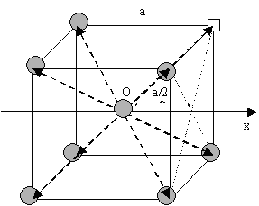
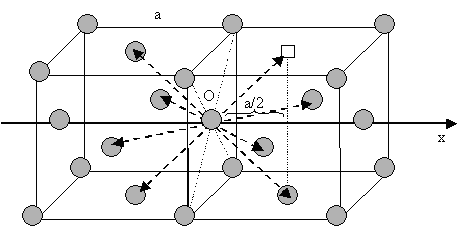
In an isotrop crystal with body centred cubic (BCC) structure (or face centred cubic — FCC), the jumping lengths and frequencies are the same for the $$8$$ (FCC: $$12$$) directions [see Figure (BCC) and Figure (FCC) ]. Applying relation \eqref{eq:Dx} for the direction Ox, one can write for both of the structure types:

\begin{equation}
D_x=\frac{1}{2}8\left(\frac{a}{2}\right)^2 = \Gamma_sa^2.
\end{equation}

2.4 Interdiffusion

If we contact two materials, let’s say $$A$$ and $$B$$, the $$A$$ atoms start to enter into the $$B$$ material, whereas the $$B$$ atoms to the $$A$$. This phenomenon is called interdiffusion. The mixing process continues until the system reaches its equilibrium state in which the atoms are distributed completely randomly if $$A$$ and $$B$$ forms completely miscible alloy. (see Fig. completely miscible )

In principle this kind of a process can be described by Fick’s equations (see sec. Fick’s equations), i.e. Boltzmann’s transformation (see sec. Boltzmann’s transformation, parabolic law) can be applied (until the boundary conditions are valid). Consequently, a plane with constant composition shifts proportionally to the square root of the time, which also means that the thickness of the diffusion zone is also $$\propto \sqrt{t}$$. (see Fig. parabolic law)

If the system has a tendency for phase separation, the intermixing stops when the initially pure materials cannot solve more impurity atoms, i.e. when the impurity concentration reaches the solubility limit. (see Fig. phase separating) In this state the impurity atoms are distributed completely randomly on both side of the interface but the composition is different.

If the system favors ordering, the atoms are not distributed randomly but tend to form a well defined chemical order (stoichiometric order). For instance, if the stoichiometric composition is $$A_{50\%}B_{50\%}$$ and the lattice is BCC, an $$A$$ atom wants to have has only $$B$$ neighbors and vica-versa. Consequently, the atoms in the diffusion zone are ordered form the beginning of the process and the width of this ordered zone growths in time until the atoms are completely ordered in the whole sample. (see Fig. ordering)

2.4.1 Atomic fluxes

According to the Onsager’s theorem, in an $$A/B$$ binary system, if the only driving force is the gradient of the chemical potential ($$\mu_i$$), the flux of $$i$$ ($$A$$, $$B$$) atoms relative to the lattice planes can be given as:

\begin{equation}
\vec{j_i}=-L_{ii}\mathrm{grad}\mu_i \label{eq:onsager}
\end{equation}

where $$L_{ii}$$ is the ‘Onsager coefficient’. The chemical potential can be expressed in the following way:

\begin{equation}
\vec{\mu_i}=\mu_0+k_bT\ln \gamma_i c_i, \label{eq:mu}
\end{equation}

where $$k_B$$ is Bolzmann’s constant and $$T$$ the absolute temperature. Moreover, $$c_i$$ and $$\gamma_i$$ are the atomic fraction and the thermodynamic activity coefficient, respectively. Combining equations (\ref{eq:onsager}) and (\ref{eq:mu}) and using that $$\rho_i\partial c_i/\partial\rho_i=c_i$$ and $$\rho_a+\rho_B=\rho=\mathrm{conts}$$, one obtains:

\begin{equation}
\vec{j_i}=-\frac{k_BTL_{ii}}{\rho_i}\left[1+\frac{\partial\ln\gamma_i}{\partial\ln
c_i}\right]\mathrm{grad}\rho_i=-\frac{k_BTL_{ii}}{\rho_i}\Theta\mathrm{grad}\rho_i=-D_i\mathrm{grad}\rho_i, \label{eq:Onsager_flux}
\end{equation}

where $$\Theta$$ is the thermodynamic factor. $$D_i$$ is the intrinsic diffusion coefficient which relates to the Brownian diffusion coefficient $$D^i$$ (see section Atomic aspects of volume diffusion) by $$\theta$$:

\begin{equation}
D_i=\Theta D^i.
\end{equation}

2.4.2 Interdiffusion coefficient, Kirkendall effect

When two species of atoms intermingle, their rate of mixing depends on the diffusion rates of both species. For diffusion in an isolated system, an interdiffusion coefficient (or mutual diffusion coefficient or chemical diffusion coefficient) can be defined, which gives the rate at which the original concentration gradient disappears.

When the two species in an interdiffusion experiment have unequal intrinsic diffusion coefficients, there is a net atom flux across any plane in the diffusion zone. Thus, more atoms will be on one side of the interface after diffusion which results a net volume transport. This is equivalent to the creation of a non-uniform stress-free strain: on one side of the diffusion zone contractions, while on the other side extractions will arise. The stress field related to this stress-free strain contributes to the atomic fluxes across the driving force $$-\Omega\mathrm{grad} p$$, and could cause a plastic deformation (by creep or by dislocation glide) as well. The plastic flow obviously relaxes the stress developed and results in a complex feed-back effect. The description of the interdiffusion process then depends on the ratio of the relaxation time of plastic flow, $$\tau$$, and the time of diffusion $$t$$.

If $$t \gg \tau$$ the relaxation of stress can be considered to be fast and almost complete. In this case the stress gradient as a driving force can be neglected. However, the relaxation of stresses is equivalent to a convective transport in the diffusion zone: e.g. for vacancy mechanism, expansion as well as contractions on different sides of the diffusion zone can be realized by annihilation and creation of vacancies at edge dislocations. From experimental point of view, if there is no change in the lateral dimensions of the specimens, a marker wire introduced originally at the interface appears to move toward one end of the diffusion couple. This effect, which was first observed by Kirkendall is called the Kirkendall shift (see Fig. Kirkendall).

The marker wire is assumed to identify a given lattice plane. The flux $$\vec{j_i}$$ of $$i$$ ($$A$$, $$B$$) species with respect to a given lattice plane (in the lattice frame) can be expressed in terms of intrinsic diffusion coefficients as in equation (\ref{eq:Onsager_flux}). If the plane is moving with velocity $$\vec{v}$$ with respect to the ends of the diffusion couple (in the laboratory frame of reference), the flux of $$\vec{j’_i}$$ $$i$$ ($$A$$, $$B$$) species with respect to the ends of the diffusion couple is:

\begin{equation}
\vec{j’_i}(\vec{r},t)=\vec{j_i}(\vec{r},t)+\rho_i(\vec{r},t)\vec{v}(\vec{r},t). \label{eq:j_i_prime}
\end{equation}

In a two component crystal of constant dimensions and atom density (the number of lattice sites is conserved, i.e. $$\partial(\rho_a+\rho_B)/\partial t=0$$), it is necessarily true that $$\vec{j’_A}=\vec{j’_B}$$ and $$\partial c_A/\partial x=-\partial c_B/\partial x)$$. Thus the total atom flux $$\vec{j’_t}$$ with respect to the ends of the couple is:

\begin{equation}
\vec{j’_t}=\vec{j’_A}+\vec{j’_B}=-\left(D_A-D_B\right)\mathrm{grad}\rho_A+\rho \vec{v}=0. \label{eq:j_total_prime}
\end{equation}

The Kirkendall velocity can then be written in the following form:

\begin{equation}
\vec{v}=\frac{1}{\rho}\left(D_A-D_B\right)\mathrm{grad}\rho_A.
\end{equation}

Therefore, using equations (\ref{eq:Fick_I}), (\ref{eq:j_i_prime}) and (\ref{eq:j_total_prime}) the fluxes of $$A$$ and $$B$$ atoms can be expressed by:

\begin{equation}
\vec{j’_A}=-\vec{j’_B}\frac{1}{\rho}\left(\rho_B D_A + \rho_A D_B\right)\mathrm{grad}\rho_A.
\end{equation}

Consequently, the interdiffusion can be characterised by only one diffusion coefficient defined in the following way:

\begin{equation}
\tilde{D}:=\frac{1}{\rho}\left(\rho_B D_A + \rho_A D_B\right)=c_B D_A + c_A
D_B, \label{eq:Darken_formula}
\end{equation}

where $$c_i = \rho_i/\rho$$ ($$i = A,B$$) is the atomic fraction. Equation (\ref{eq:Darken_formula}) is called as Darken’s formula.

On the other hand, if $$t \ll \tau$$ (but $$t$$ is long enough for the development of the stress gradient) then we can be in a second limit, when practically there is no stress relaxation at all ($$\vec{v} \approx 0$$ ). An additional term proportional to the stress (pressure) gradient should be added to the right hand side of equation (\ref{eq:Fick_I}) and it can be shown that the mixing process is controlled by:

\begin{equation}
\tilde{D}_{NP}:=\frac{D_AD_B}{c_AD_A+c_AD_B}. \label{eq:Nernts_Planck}
\end{equation}

Here the index NP indicates that this is the so-called Nernst-Planck limit. After an initial transient period the pressure gradient developed makes the two fluxes equal, i.e. the volume transport will be determined by the slower intrinsic diffusion coefficient (series coupling of currents) in contrast to the Darken’s limit (parallel coupling), where the chemical diffusion coefficient is determined by the faster one.

2.5 Composition dependent diffusion coefficient — Diffusion asymmetry

Usually the tracer (or Brownian) diffusion coefficient of a diffusion specie is different on the two sides of a diffusion couple (diffusion asymmetry). (see Fig. diffusion asymmetry) This originates from the difference in the bonding strength in the different matrixes. Therefore, the jump probabilities of the atoms or the diffusion coefficient depend on the local environment, i.e. on the local composition.

The interface in a diffusion couple is usually not atomically sharp but more or less diffused. This means that the composition changes, consequently the diffusivity also changes accordingly. Therefore the (tracer) diffusion coefficients are composition dependent.(see Fig. composition dependent diffusivity) (for this reason the \eqref{eq:constD_Fick_II} form of Fick’s second law is not advised)

The composition dependence of the diffusion coefficient ($$D$$) or the jump frequency ($$\Gamma$$) can be considered in both continuum and atomic models, for instance, in the following form: $$D = D_0 \exp(mc)$$ or $$\Gamma = \Gamma_0 \exp(mc)$$, where $$D_0$$ and $$\Gamma_0$$ are composition independent pre-exponential factors, $$c$$ is the composition of one of the constituents (e.g. of $$A$$) and $$m$$ is a parameter determining the strength of the composition dependence. It is worth introducing an $$m’ = m \log_{10}e$$ ($$e$$ is the base of natural logarithm) parameter, since thus $$\log_{10}(D/D_0) = \log_{10}(\Gamma/\Gamma_0) = m’c$$, i.e its value gives in orders of magnitude the ratio of the jump probabilities or diffusion coefficients in the pure $$A$$ and $$B$$ matrixes. (see Fig. definition of m’) This gives the possibility to determined $$m’$$ experimentally from the self and impurity diffusion coefficients (and can also be called as diffusion asymmetry parameter). [ErdelyiPhilMag1999] Note that, $$m’$$ can also be derived from the difference in the $$A-A$$ and $$B-B$$ pair interaction energies (see e.g.  Ref. [ErdelyiPhilMag1999]). If $$m’$$ is positive/negative, the jumps are faster/slower in the $$B$$ matrix. For instance, $$m’ = 4$$ means that the jumps are $$10,000$$ times faster in the $$B$$ matrix than in $$A$$. The ratio of the diffusion coefficients is usually several orders of magnitude ($$4-7$$). The diffusion asymmetry is seldom considered despite that in nature usually different atoms have different mobility in different materials.

The animation in Fig. definition of m’ (animated) illustrates how the diffusivity of an $$A$$ ($$B$$) atom changes while it diffuse from the $$A$$ ($$B$$) matrix to the $$B$$ ($$A$$).

Remark: Usually we, suppose that the diffusion coefficient has exponential composition dependence. However, it is not obligatory, any kind of function may be assumed, it does not alter the general conclusions.

2.6 Discrete / atomistic models

In case of continuum models, it is easy to consider the diffusion asymmetry. We have just to suppose the diffusion coefficients to be composition dependent: $$D=D(c)$$, e.g. $$D=D_0\exp(mc)$$. However, in case of atomistic models, the composition dependence of the jump frequencies or jump probabilities needs more considerations.

2.6.1 One dimensional kinetic mean filed model (KMF)

Our model to calculate the time evolution of the composition on a one-dimensional lattice is based on Martin’s equations. [MartinPRB1990] However, we use our own composition dependent activation barriers (diffusion asymmetry) in the exchange frequencies, which unify the advantages of other barriers used in the literature as was shown in Ref. [ErdelyiPRB702004]. The time derivatives of atomic fractions of $$A$$ atoms in the $$i$$-th atomic layer perpendicular to the $$x$$-axis can be given by:

Here $$J_{i,i+1}$$ is the net flux of $$A$$ atoms from plane $$i$$ to $$(i+1)$$:

\begin{equation}
J_{i,i+1}=z_v \left[ c_i(1-c_{i+1}) \Gamma_{i,i+1}-
c_{i+1}(1-c_i) \Gamma_{i+1,i} \right],
\end{equation}

where $$c_i$$ is the atomic fraction of A atoms in plane $$i$$, $$\Gamma_{i,i+1}$$ is the frequency with which an A atom in plane $$i$$ exchanges with a B atom in plane $$i+1$$ and $$z_v$$ is the vertical coordination number. It is usually assumed that the exchange frequencies have an Arrhenius type temperature dependence:

\begin{equation}
\Gamma_{i,i+1}=\Gamma_i \gamma_i
\text{ and }
\Gamma_{i+1,i}=\Gamma_i/ \gamma_i
\end{equation}

with

\begin{equation}
\Gamma_i=\Gamma_0\exp[\alpha_i/kT]
\text{ and }
\gamma_i=\exp[-\varepsilon_i/kT],
\end{equation}

were $$\Gamma_0=\nu\exp[-\hat E_0/kT]$$, $$\nu$$ denotes the attempt frequency, $$\hat E_0$$ is composition independent and contains the saddle point energy, $$k$$ is the Boltzmann constant, $$T$$ is the absolute temperature, and

\begin{equation}
\alpha_{i}=\left[z_{v}(c_{i-1}+c_{i+1}+c_{i}+c_{i+2})+z_{l}(c_{i}+c_{i+1})\right]M
\end{equation}

as well as

\begin{equation}
\varepsilon_{i}=\left[z_{v}(c_{i-1}+c_{i+1}-c_{i}-c_{i+2})+z_{l}(c_{i}-c_{i+1})\right]V.
\end{equation}

Here $$z_l$$ is the lateral coordination number, $$V$$ is the same regular solid solution parameter as in KMC, and also similarly to the KMC model, $$M$$ measures the diffusion asymmetry. Here $$m’=-2ZM/kT\log_{10}e$$, where $$e$$ is the base of natural logarithm and $$(Z= 2z_v + z_l)$$. [ErdelyiPRB702004]

The input parameters in the model are, therefore: [ErdelyiPRB702004] $$V$$ regular solid solution parameter; $$T$$ temperature; $$z_v$$, $$z_l$$ vertical and lateral coordination numbers [$$z_v=4$$, $$z_l=0$$ for a BCC structure and $$z_v=4$$, $$z_l=4$$ for an FCC structure in (100) direction]; and $$m’$$ diffusion asymmetry parameter.

2.6.2 Three dimensional kinetic Monte Carlo model (KMC)

Monte Carlo simulations of the kinetic process can be performed using for instance the residence-time algorithm. [SoissonActaMat1996] It is quite common to use the so-called one-vacancy model, when there is always one vacancy in the simulation box. In this case, for comparison to real time scale, the simulation time should be rescaled to corresponding real concentrations.

If only atom-vacancy exchange is allowed, the exchange probability of a vacancy-atom pair can be calculated from the binding energy of the atom. This energy can be calculated easily in a simple nearest-neighbour interaction approximation either for an $$A$$ ($$E_A$$) or $$B$$ ($$E_B$$) atom:

\begin{eqnarray}
E_A &=& n_A V_{AA} + n_B V_{AB}, \notag \\
E_B &=& n_A V_{AB} + n_B V_{BB},
\label{eq:E}
\end{eqnarray}

where $$n_A$$ and $$n_B$$ are the number of $$A$$ and $$B$$ atoms in the vicinity of the given atom, $$V_{ij}$$ ($$i,j=A$$ or $$B$$) is the interaction energy between an $$ij$$ atom pair. Introducing $$V = V_{AB} – \frac{V_{AA}+V_{BB}}{2}$$ and $$M = \frac{V_{AA} – V_{BB}}{2}$$, Eqs.~\eqref{eq:E} can be written as:

\begin{eqnarray}
E_A &=& -n_A (V-M) + n V_{AB}, \notag \\
E_B &=& -(n-n_A) (V+M) + n V_{AB}.
\end{eqnarray}

where $$n=n_A+n_B$$ is the number of neighbors of an atom, $$V$$, is the regular solid solution parameter [proportional to the mixing energy and measures the phase separating $$(V>0)$$ or ordering $$(V<0)$$ tendency] and $$M$$ measures the diffusion asymmetry ($$m’=-2nM/kT\log_{10}e$$, where $$e$$ is the base of natural logarithm). [ErdelyiPRB702004] Using the usual Arrhenius-relationship between the activation energy ($$Q_i=E^0-E_i$$, where $$E^{0}$$ is the saddle point energy, and $$i=A,B$$) and the probability [$$\Gamma_{iV} = \nu \exp(-Q_i/kT)$$], the exchange probabilities of a vacancy-$$i$$ atom pair are:

\begin{eqnarray}
\Gamma_{VA} &=& \nu \exp \left[-\frac{\hat{E}^{0}+n_A (V-M)}{kT}\right], \notag \\
\Gamma_{VB} &=& \nu \exp \left[-\frac{\hat{E}^{0}+(n-n_A) (V+M)}{kT}\right],
\end{eqnarray}

where $$k$$ and $$T$$ are the Botzmann’s constant and the absolute temperature, $$\nu$$ is the attempt frequency, and $$\hat{E}^0 = -E^0 + nV_{AB}$$. Note that $$\hat{E}^0$$ is taken to be constant for a given system, and thus it may be set to zero during calculations (but can be considered in the time scaling if needed).